Visualize Direction of Relationships
Contents
Visualize Direction of Relationships
The correlation falls between -1 and 1 (\(-1 \leq r_{xy} \leq 1\)).
If \(r_{xy} > 0\), the association is positive,
If \(r_{xy} < 0\), the association is negative, and
If \(r_{xy} = 0\), it indicates no linear relationship.
The larger the absolute value \(r_{xy}\), the stronger the association.
Let’s investigate how the scatter plot changes as the correlation changes.
# Importing the necessary libraries
import warnings
warnings.filterwarnings("ignore")
import ipywidgets as widgets
import numpy as np
import pandas as pd
import matplotlib.pyplot as plt
import scipy.stats as stats

plt.style.use('seaborn-whitegrid')
plt.rcParams['figure.figsize']=14,6

# define a corr function with flexible corr input
def corr_widget(corr = 0):

    # Defining the mean vector
    mean_x_y = np.array([20,30])

    # Setting sd and corr

    sigma_x = 4
    sigma_y = 5
    corr_x_y = corr

    # Defining the variance-covariance matrix

    cov_x_y = np.array([[sigma_x**2, corr_x_y*sigma_x*sigma_y], [corr_x_y*sigma_x*sigma_y, sigma_y**2]])

    # Generating a data based on bivariate normal distribution
    # with given mean vector and variance-covariance matrix

    data = stats.multivariate_normal.rvs(mean = mean_x_y, cov = cov_x_y, size = 100)

    # Plotting the generated samples

    plt.plot(data[:,0],data[:,1], 'o', c='blue')
    plt.title(f'Correlation between X and Y = {corr_x_y}')
    plt.xlabel('X')
    plt.ylabel('Y')

    plt.show()

#turn it into a widget
corr_wid = widgets.FloatSlider(min = -1, max = 1, step=0.1, value=0, description = "$r_x_y$")
#display(corr_wid)
Now, play with the follwing slider to see how correlation changes.
widgets.interact(corr_widget, corr = corr_wid);
Example
An educational economist may want to build the relationship between an individual’s income (in $) and education (in years).
S/he takes a random sample of 10 individuals and asks for their income (in $1000s) and education (in years).
The results are shown below:
#present data
data = {'Education': [11,12,13,15,8,10,11,12,17,11],
        'Income': [25,27,30,41,18,23,26,24,48,26]}
data
{'Education': [11, 12, 13, 15, 8, 10, 11, 12, 17, 11],
 'Income': [25, 27, 30, 41, 18, 23, 26, 24, 48, 26]}
# plot education vs income to explore the relationship
plt.style.use('seaborn-whitegrid')
plt.plot(data['Education'],data['Income'], 'o', c='blue')
plt.xlim([np.min(data['Education'])-1, np.max(data['Education'])+1])
plt.xlabel('Education in years')
plt.ylabel('Income in $')
plt.show()
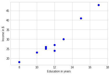
The scatter plot between the education (in years) and income (in dollars) shows a linear relationship. Let’s compute the sample correlation coefficient \(r_{xy}\) between the education and income.
# get the corr between education and income
corr = np.corrcoef(data['Education'],data['Income'])
# Print the result
print(corr)
[[1.        0.9651672]
 [0.9651672 1.       ]]
This indicates a strong and positive linear relationship between Education in years and Income.
Session Info
import session_info
session_info.show()
Click to view session information
-----
ipywidgets          7.7.0
matplotlib          3.5.2
numpy               1.22.4
pandas              1.4.2
scipy               1.8.1
session_info        1.0.0
-----
Click to view modules imported as dependencies
PIL                 9.1.1
asttokens           NA
backcall            0.2.0
beta_ufunc          NA
binom_ufunc         NA
cffi                1.15.0
colorama            0.4.4
cycler              0.10.0
cython_runtime      NA
dateutil            2.8.2
debugpy             1.6.0
decorator           5.1.1
defusedxml          0.7.1
entrypoints         0.4
executing           0.8.3
hypergeom_ufunc     NA
ipykernel           6.13.0
ipython_genutils    0.2.0
jedi                0.18.1
kiwisolver          1.4.2
matplotlib_inline   NA
mpl_toolkits        NA
nbinom_ufunc        NA
packaging           21.3
parso               0.8.3
pexpect             4.8.0
pickleshare         0.7.5
pkg_resources       NA
prompt_toolkit      3.0.29
psutil              5.9.1
ptyprocess          0.7.0
pure_eval           0.2.2
pydev_ipython       NA
pydevconsole        NA
pydevd              2.8.0
pydevd_file_utils   NA
pydevd_plugins      NA
pydevd_tracing      NA
pygments            2.12.0
pyparsing           3.0.9
pytz                2022.1
six                 1.16.0
sphinxcontrib       NA
stack_data          0.2.0
tornado             6.1
traitlets           5.2.1.post0
wcwidth             0.2.5
zmq                 23.0.0
-----
IPython             8.4.0
jupyter_client      7.3.1
jupyter_core        4.10.0
notebook            6.4.11
-----
Python 3.8.12 (default, May  4 2022, 08:13:04) [GCC 9.4.0]
Linux-5.13.0-1023-azure-x86_64-with-glibc2.2.5
-----
Session information updated at 2022-05-28 16:28