MLE for Normal Distribution
MLE for Normal Distribution
Let’s work on how we can find MLE under normal distribution.
import warnings
warnings.filterwarnings("ignore")
#import required libraries
import pandas as pd
import numpy as np
import scipy.stats as stats
import matplotlib.pyplot as plt
import math
For this case, let’s generate a synthetic sample of size n=100 from N(0,1).
#let's generate a synthetic observed sample
data = stats.norm.rvs(loc = 0, scale = 1, size = 100)
n = np.size(data)
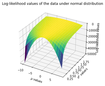
Since we a parameter vector (\(\mu\) and \(\sigma^2\)) now, we will create 3D plot where X-axis will be for possible \(\mu\) values, Y-axis will be for possible \(\sigma^2\) values, and Z-axis will be the corresponding log-likelihood value for the sample under given \(\mu\) and \(\sigma^2\).
# Generate a meshgrid
# A vector grid for possible mu values
mu_values = np.arange(-10,10,1)
# A vector grid for possible sigma2 values
sigma2_values = np.arange(0.1,2,0.1)
# Create coordinate points of X and Y
X, Y = np.meshgrid(mu_values, sigma2_values)
Calculate the loglikelihood value of normal distribution for each possible \(\mu\) and \(\sigma^2\).
# Estimate the log-lik function of normal distribution for each point mu and sigma2 value in the meshgrid
loglik = np.zeros(X.shape)
for i in range(X.shape[0]):
    for j in range(X.shape[1]):
        loglik[i,j] = -(n/2)*np.log(2*math.pi*Y[i,j])-(1/(2*Y[i,j]))*np.sum((data-X[i,j])**2)
#double check for loop calculations
#loglikfake = -(n/2)*np.log(2*math.pi*sigma2_values[0])-(1/(2*sigma2_values[0]))*np.sum((data-mu_values[0])**2)
#loglikfake
# Plotting the log-lik values
fig = plt.figure(figsize=plt.figaspect(5))
ax = fig.add_subplot(1, 1, 1, projection='3d')
ax.plot_surface(X, Y, loglik, cmap = 'viridis')
plt.xlabel(r'$\mu$ values')
plt.ylabel(r'$\sigma^2$ values')
plt.title('Log-likelihood values of the data under normal distribution')
ax.set_zlabel('Log-likelihood values', rotation=80)
ax.set_zlim(-50000, 0) #limits are manually set
plt.tight_layout()
plt.show()
We can also find the maximum (minimum) point where the log-likelihood (negative log-likelihood) attains through an optimization routine. First define neg-log-lik as a function. Then use minimize() function fom Scipy.optimize with method='L-BFGS-B' to find the arg min.
def normal_negloglik(param):

    mu = param[0]
    sigma2 = param[1]

    #data is not an input argument, assuming data object is already available in the session.
    #fixed values
    n = np.size(data)

    #define log_likelihood
    log_lik = -(n/2)*np.log(2*math.pi*sigma2)-(1/(2*sigma2))*np.sum((data-mu)**2)

    neg_log_lik = -log_lik

    return neg_log_lik
from scipy.optimize import minimize
normal_mle = minimize(normal_negloglik, np.array([1,1]), method='L-BFGS-B')
normal_mle
      fun: 155.31917177807796
 hess_inv: <2x2 LbfgsInvHessProduct with dtype=float64>
      jac: array([-5.68434189e-06,  2.84217096e-06])
  message: 'CONVERGENCE: NORM_OF_PROJECTED_GRADIENT_<=_PGTOL'
     nfev: 27
      nit: 8
     njev: 9
   status: 0
  success: True
        x: array([0.04046438, 1.3080093 ])
Actually those values are \(\hat \mu = \bar X\) and \(\hat \sigma^2 = \frac{\sum_{i=1}^{n=100}(x_i-\bar x)^2}{n}\). See below.
np.mean(data)
0.040464447281173245
np.sum((data-np.mean(data))**2)/np.shape(data)
array([1.30800931])