Consistency of Sample Mean
Consistency of Sample Mean
Assume that we have a random sample of size n from a population with \(N(\mu, \sigma^2)\). Let’s investigate how the probability \(Pr(|\bar{X}_{n}-\mu| > \epsilon)\) changes with respect to n and \(\epsilon\) and, when \(\sigma^2 = 4\).
Note that due to symmetry of normal distribution, \(Pr(|\bar{X}_{n}-\mu| > \epsilon) = 2 Pr\big(Z > \frac{\epsilon}{\sigma /\sqrt n}\big)\).
# import required libraries
import numpy as np
import scipy.stats as stats
import matplotlib.pyplot as plt
from IPython.display import display
def xbar_consistency(eps, col):

    #fixed
    sigma = 2

    fig, ax = plt.subplots(figsize = (6, 6))

    for e, cl in zip(eps, col):
        samp_size = np.arange(1, 101, 1)
        #calculate the probability under given settings
        prob = 2*(1-stats.norm.cdf(x = e*np.sqrt(samp_size)/sigma, loc = 0, scale = 1))
        #plot
        plt.plot(samp_size, prob, c = cl, label = r'$\epsilon=%.1f$' % (e))

    plt.xlim(0, 101)
    plt.ylim(0, 1)
    plt.xlabel(r'Sample size')
    plt.ylabel(r'$Pr(|\bar{X}_{n}-\mu| > \epsilon)$')
    plt.title('Probabilities with respect to n and $\epsilon$')
    plt.legend(loc='upper right')
    plt.show()
eps_values = [0.1, 0.25, 0.5, 1]
col_values = ['black', 'red', 'blue', 'green']
xbar_consistency(eps = eps_values, col = col_values)
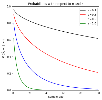
For a given \(\epsilon\) value, the probability \(Pr(|\bar{X}_{n}-\mu| > \epsilon)\) forms a sequence and it decreases towards zero as we increase the sample size \(n\). When we change the value of maximum difference, \(\epsilon\).
We can also investigate how the complementary probability, namely, \(Pr(|\bar{X}_{n}-\mu| < \epsilon)\) changes with respect to n and \(\epsilon\) and , when \(\sigma^2 = 4\).
def xbar_consistency_toone(eps, col):

    #fixed
    sigma = 2

    fig, ax = plt.subplots(figsize = (6, 6))

    for e, cl in zip(eps, col):
        samp_size = np.arange(1, 101, 1)
        #calculate the probability under given settings
        prob1 = 2*(1-stats.norm.cdf(x = e*np.sqrt(samp_size)/sigma, loc = 0, scale = 1))
        prob = 1-prob1
        #plot
        plt.plot(samp_size, prob, c = cl, label = r'$\epsilon=%.1f$' % (e))

    plt.xlim(0, 101)
    plt.ylim(0, 1)
    plt.xlabel(r'$Sample size$')
    plt.ylabel(r'$Pr(|\bar{X}_{n}-\mu| < \epsilon)$')
    plt.title('Probabilities with respect to n and $\epsilon$')
    plt.legend(loc='upper right')
    plt.show()
eps_values = [0.1, 0.25, 0.5, 1]
col_values = ['black', 'red', 'blue', 'green']
xbar_consistency_toone(eps = eps_values, col = col_values)
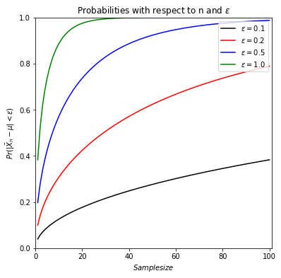
Similarly, for a given \(\epsilon\) value, the probability \(Pr(|\bar{X}_{n}-\mu| < \epsilon)\) forms a sequence and it increases towards one as we increase the sample size \(n\). For a given sample size, when we change the value of maximum difference, \(\epsilon_1\) to \(\epsilon_2\) (\(\epsilon_1 < \epsilon_2\)),we see that \(Pr(|\bar{X}_{n}-\mu| < \epsilon_1) < Pr(|\bar{X}_{n}-\mu| < \epsilon_2)\) which makes sense that falling into a wider a wider interval results in a higher probability.